3. Use of HRLoad
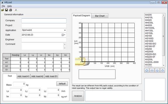
Figure 3.1 HRLoad execution screen
When HRLoad is started, the screen will be displayed as shown in Figure 3.1. First of all, you need to enter 『General Information』 on the upper left. The entered values will be recorded together with the report that will be printed out later, while the values will not make any influence on the results of the analysis.

Figure 3.2 Entering of Generation Information
As next, you need to enter the 『Tool』 and the『Additive load values』 on the lower left. The analysis results will be influenced by these entered values. There are 4 different tabs, one for the tool that will be mounted on the robot’s flange, and three for the 『Additive loads (V, H, and S)』 that will be mounted on the 3 links.

Figure 3.3 A dialogue box for entering the load data
An additive load is the load that will be mounted on the link, not on the robot’s tool flange. A servogun dress pack or a cable guide is one of the examples.
In each tab, there are items that need to be entered as shown in Table 3-1. They include weight, center of mass and moment of inertia. Users should enter the values for all tabs (If there is not additive load, “0’ just needs to be set all for the relevant tabs).
Table 3‑1 Items to be entered for the load
Items | Description | Unit |
Weight | Weight of the load mounted on the robot | kg |
Lx, Ly, Lz | Position of the center of mass of the load | mm |
Ixx, Iyy, Izz | Moment of inertia of the load | kg m2 |
Selecting the coordinate system from the help menu or clicking the tool button in the shape of the coordinate system on it, users can get the information about the positions of the coordinate system and additive load.
 à
à 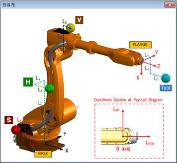
Figure 3.4 The coordinate system and the positions of additive load
It is time to select a robot. Select a robot from the list on the left, and then click the “+” button at the bottom of the list. A name of a robot will be added to the legend linked to a graph (Max. 3 names can be added). In order to delete a name, select the robot in the legend and then click “-” button.
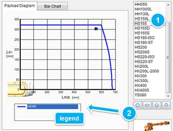
Figure 3.5 Adding a robot to the legend
(Can change the color by changing the order of the robots in the legend by using the Up/Down arrow buttons).
As a last step, when the analysis button at the bottom is clicked, the calculation will be completed. Let’s take a look at the 『Payload Diagram』 first. We now know that the star mark stays inside the graph. This means that, statistically, overweight will not be caused.
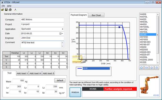
Figure 3.6 Analysis results - Payload Diagram
As next, click the 『Bar Chart』 tab. We now know that the load for the J6 axis (The sixth axis, in other words, the R1 axis) exceeds the max. allowable value of 100%.
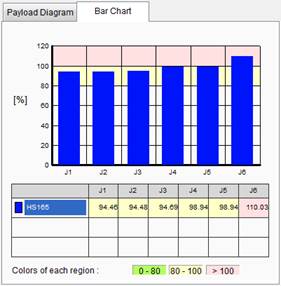
Figure 3.7 Analysis results - Bar Chart
The final results will be produced on the right side of the analysis button. In terms of statistics, the robot has no problem. However, considering that the robot is in the dynamical overweight state, if the robot needs to be used despite the fact, it may be required to slow down the speed of it due to the overweight error, following the installation. The meaning of the final conclusion, see Table 3-2.

Figure 3.8 Analysis results - Final conclusion
Table 3‑2 Meaning of the final conclusion
Massage | Ground color | Payload Diagram | Bar Chart | Conclusion |
PASSED | Green | Within the allowed area J | All the axes below 100%, the max. allowed level J | Can be operated at normal speeds |
Further analysis required | Red | Within the allowed area J | Some axes above 100%, the max. allowed level L | Limited operation through the adjustment of the max. speed. |
UNPASSED | Red | Exceeding the allowed area L | Don’t care | Not allowed to use |
In the above example, it is found that the HS165 model has the possibility of overweight. Now, it time to make comparison with other robots with higher payloads. Add the HS180-ST and HS200 to the legend by using the “+” button. Push the button to run the calculation for the 3 models. While the 『Payload Diagram』 and the『Bar Chart』 will show the results of multiple models together, the final results will show the information only about the robot that is currently selected from the legend.
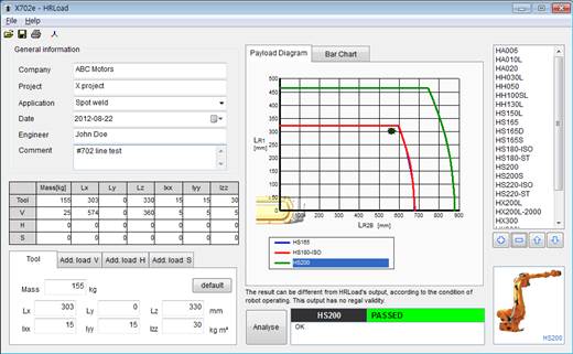
Figure 3.9 Comparison of robot models
In this example, as there is almost no difference between HS165 and HS180-ST, whose graphs are almost overlapped, while the graph for HS200 shows a wider scope. According to the 『Payload Diagram』, all the 3 robot models are not in the overweight state.
The 『Bar Chart』 shows that HS165 and HS180-ISO exceed 100% at the J6 bar, meaning that overweight is expected. In case of HS200, all the six bars are below 80% as we can see. When HS200 is selected from the legend, the final result will be indicated as PASSED.
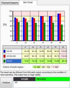
Figure 3.10 Comparison of robot models - Bar chart and final conclusion
Selecting the “file – save” menu will allow the entered data to be saved as a file with the extension of ‘.hrload’. It can be retrieved by using the “file – open” menu later (It is also possible to drag and drop a ‘.hrload’ file onto HRLoad).
Selecting the “file – print” menu or clicking the print tool button will bring up a dialogue box. Select a printer at the upper part and click the print button to print out a report.
In case of a color printer, the Gray-scaled check button needs to be turned off to print the report in colors.
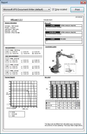
Figure 3.11 Report printing-out function